A Technical Deep-Dive into AI-Powered Archery Score Detection

Archery scoring is deceptively tedious. After every “end” (a set of 3 or 6 arrows), an archer walks to the target, reads each arrow’s position by eye, announces the score to a recorder, pulls the arrows, and walks back. Multiply that by 20+ ends in a competition and you have a process that is slow, fatigue-prone, and entirely dependent on human judgment for calls near ring boundaries.

The goal of this project was straightforward: photograph the target, get the scores back instantly. But making that work reliably across different lighting conditions, camera angles, arrow densities, and target sizes turned out to involve a non-trivial set of problems, dataset engineering, model selection, perspective geometry, and a custom scoring engine. This post covers every decision in full detail.

The full code is available on GitHub.

---

Table of Contents

• Project Vision & Scope
• Data Engineering & Methodology
• Model Architecture: YOLO26
• Training Hyperparameters — Every Setting Explained
• Performance Metrics — What They Mean in This Context
• Performance Results & Full Analysis
• Scoring Logic & Integration Pipeline
• Limitations, Known Issues & What’s Next

---

Project Vision & Scope

The core objective is the automation of the scoring pipeline. Traditionally, archers must walk to the target and manually record scores, a process prone to human error and fatigue. This project allows users to simply photograph the target; the AI identifies the arrows and computes their values instantly.

Target-Agnostic Design

While the MVP focuses on World Archery (WA) outdoor target faces (122cm and 80cm) using the standard 10-zone scoring system, the architectural logic is target-agnostic. By identifying universal structural markers rather than predicting static scores, the system is designed for seamless adaptation to:

• Indoor Archery: Triple-spot or 40cm faces
• Custom Targets: Proprietary club or training faces

---

Data Engineering & Methodology

A high-performance model is only as good as the data it consumes. The dataset was engineered to maintain reliability across extreme lighting conditions, various camera angles, and differing arrow densities.

Data Sourcing & Curation

I aggregated a raw pool of 3,700 images from four specialized repositories on Roboflow:

• archery-skmsa/archery^[1]
• uni-oidi4/archery^[2]
• archery-scoring/Archery Scoring^[3]
• shrutiharshil/DJS Phoenix^[4]
  

Through a rigorous **filtering phase**, I discarded low-resolution frames, redundant images, and poorly labeled samples. This resulted in a refined set of **250 high-variance images** chosen specifically for the fine-tuning phase.

Geometric Pre-processing: Segmentation → Detection

A significant challenge identified during data auditing was a label format mismatch: several classes (notably arrow_shaft) were labeled as polygons (segmentation) rather than bounding boxes (detection). To maintain consistency without the labor-intensive process of manual re-labeling, I implemented a custom Python script.

The script calculates the extreme coordinates of the polygon vertices $(x_{\min}, y_{\min}, x_{\max}, y_{\max})$ to derive the bounding box center $(c_x, c_y)$ and dimensions $(w, h)$, effectively converting segmentation masks into YOLO-compatible detection labels.

Augmentation Strategy

To increase model robustness, we applied the following augmentations via Roboflow, expanding the training set to 525 images (70/20/10 split):

• Horizontal Flip: Mirrors the target to handle different approach angles.
• Brightness (-25% to +25%): Simulates varying outdoor conditions (overcast vs. direct sun).
• Blur & Noise: Mimics low-quality smartphone sensors or slight motion blur during handheld capture.

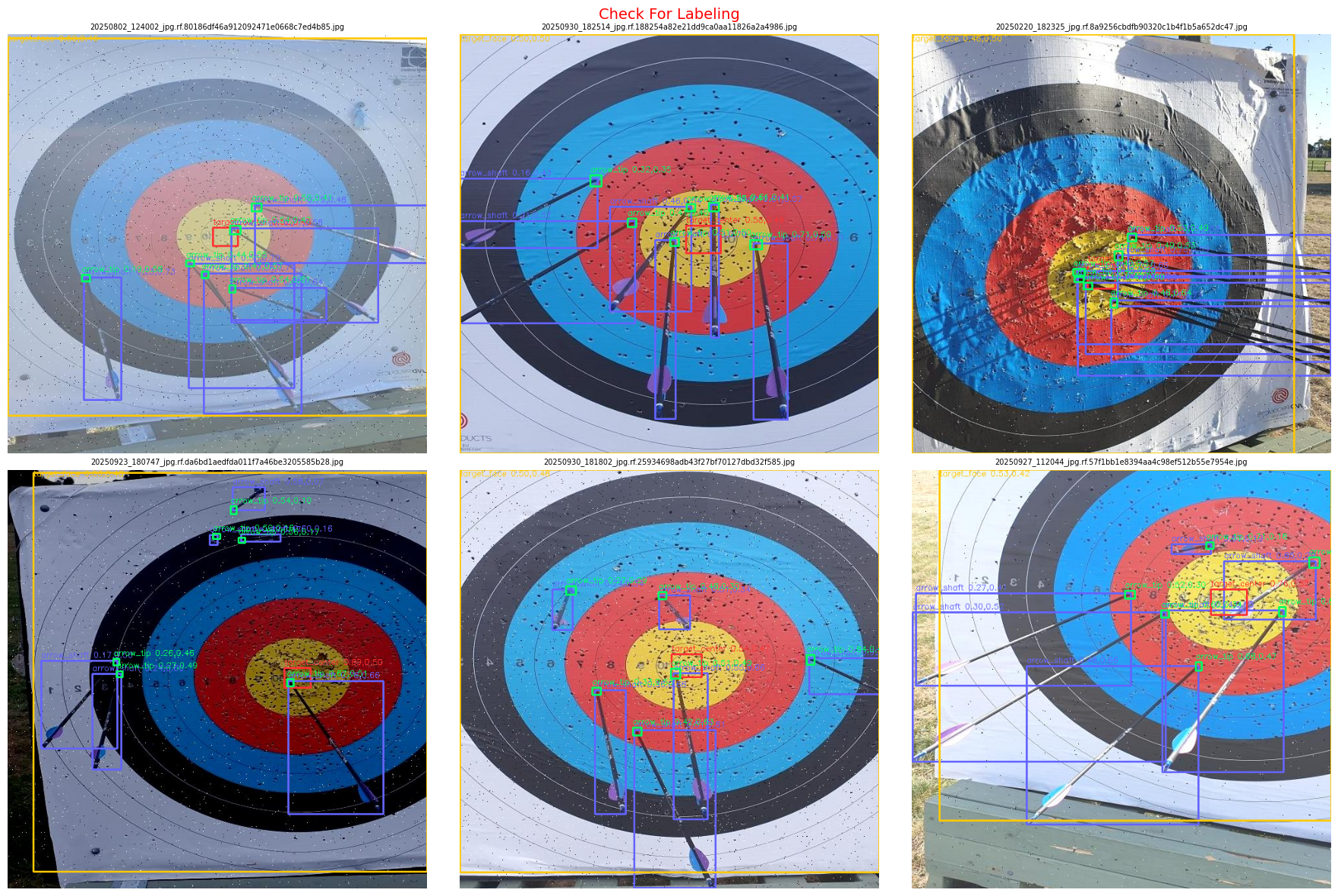
Labeling Strategy for Geometric Scoring

The four classes and their specific roles in the pipeline:

• arrow_shaft: Identifies the arrow body to assist the model in distinguishing arrows from target lines, and is used later to refine tip position via shaft direction.
• arrow_tip: The primary key for scoring, represents the precise point of impact.
• target_center: Defines the absolute origin (0,0) in the target’s coordinate system.
• target_face: A 4-point detection identifying target boundaries.

Dataset hosted on Roboflow under archeryxpert-score-detection^[5].

Class Distribution:

Class	Count
arrow_shaft	2,742
arrow_tip	2,577
target_center	519
target_face	519

---

Model Architecture: YOLO26

The project uses YOLO26^[6], the state-of-the-art standard in the YOLO family as of early 2026.

Architectural Advantages

NMS-Free (End-to-End): Traditional YOLO models use Non-Maximum Suppression to filter duplicate bounding boxes as a post-processing step. This adds latency. YOLO26 uses a direct prediction method that outputs final detections without NMS, making it significantly faster for mobile deployment.

CPU Optimization: The Nano variant (YOLO26n) is specifically tuned for edge hardware, showing a ~43% speed increase on mobile CPUs compared to YOLO11. This matters for the intended deployment target, which is a mobile app processing one image per end.

MuSGD Optimizer: By integrating Muon-style optimization (initially developed for LLM training), the model achieves more stable convergence. This is particularly important when training on smaller, specialized datasets where gradient noise is a bigger problem.

Dataset Structure

The model expects a standardized directory structure:

/images   — image files
/labels   — paired .txt files where each label contains: class_id | cx | cy | w | h
data.yaml — defines paths and class names: ['arrow_shaft', 'arrow_tip', 'target_center', 'target_face']

---

Training Hyperparameters — Every Setting Explained

epochs: 100
imgsz: 640
batch: 16
optimizer: AdamW
lr0: 0.001
lrf: 0.01
warmup_epochs: 3
weight_decay: 0.0005
hsv_h: 0.015
hsv_s: 0.7
hsv_v: 0.4
translate: 0.1
scale: 0.5
fliplr: 0.5
mosaic: 1.0
degrees: 0.0
dropout: 0.1
patience: 20
save: true
save_period: 10
plots: true
project: archery_yolo26
name: v1
exist_ok: true
device: 0
workers: 2
cache: true

Core Settings

epochs=100: One epoch means the model sees every training image once. 100 epochs means it sees every image 100 times, adjusting its weights slightly after each batch. With patience=20 it will stop early if it stops improving, so it won’t necessarily run all 100.

imgsz=640: Every image gets resized to 640×640 before the model processes it. This is fixed for the entire training run and must match at inference time. 640 is the standard, large enough to resolve small objects like arrow tips, small enough to run fast.

batch=16: Instead of processing one image at a time, it processes 16 simultaneously. Larger batches produce more stable gradient estimates and allow faster training.

Optimizer Settings

optimizer='AdamW': The algorithm that adjusts model weights after each batch. AdamW is better than the default SGD for small datasets because it adapts the learning rate per parameter automatically, essentially a smarter version of gradient descent. When you only have 500 training images, this adaptability makes a meaningful difference.

lr0=0.001: Initial learning rate — how large each weight update step is. 0.001 is a standard starting value. Too high and the model overshoots and learns nothing; too low and training takes forever.

lrf=0.01: Final learning rate as a fraction of lr0. The learning rate decays from 0.001 down to 0.001 × 0.01 = 0.00001 over the course of training. This is called learning rate scheduling, start with bigger steps to learn fast, finish with tiny steps to fine-tune precisely.

warmup_epochs=3: For the first 3 epochs, the learning rate starts near zero and gradually increases to lr0. Without warmup, the first few batches can cause large unstable weight updates that damage the entire training run. Warmup prevents this cold-start problem.

weight_decay=0.0005: L2 regularization that adds a small penalty for having large weights. This prevents overfitting by discouraging the model from memorizing training images. It keeps the model’s learned representations general rather than specialized to the specific training examples it has seen.

Augmentation Settings

These are applied randomly to training images every epoch. The model sees a slightly different version of each image every time, which artificially multiplies the dataset and teaches robustness.

hsv_h=0.015: Randomly shifts the hue by up to 1.5%. Teaches the model that slightly different-colored arrows and targets are the same thing.

hsv_s=0.7: Randomly changes saturation by up to 70%. This is a large range and is particularly important for archery, it simulates everything from vivid outdoor colors to washed-out overcast lighting. The target rings can look very different under different lighting conditions.

hsv_v=0.4: Randomly changes brightness by up to 40%. Handles the difference between indoor dim ranges and bright outdoor conditions.

translate=0.1: Randomly shifts the image up/down/left/right by up to 10% of image size. Teaches the model that objects can appear anywhere in frame, not just centered.

scale=0.5: Randomly zooms in or out by up to 50%. This is critical for archery: archers photograph from different distances. An arrow tip that’s 8px wide from 3 meters becomes 4px wide from 6 meters. This augmentation teaches the model to handle both scales correctly.

fliplr=0.5: Randomly flips the image horizontally with 50% probability. A target looks identical mirrored. An arrow shaft pointing left is the same as one pointing right. This doubles your effective dataset at zero cost.

mosaic=1.0: Takes 4 training images and combines them into a 2×2 grid, with all labels from all 4 included. This forces the model to detect objects at smaller scales and in unusual contexts. It’s one of YOLO’s most effective augmentations, essentially quadrupling training variety per step.

degrees=0.0: Rotation augmentation is explicitly set to zero because the bounding box labels aren’t drawn to handle rotation. If training images were rotated, the axis-aligned bounding boxes would stay horizontal while the actual objects inside them were tilted, giving the model incorrect supervision signals.

Regularization

dropout=0.1: During training, randomly sets 10% of neurons to zero on each forward pass. This prevents any single neuron from becoming too important and forces the network to learn redundant representations. The result is better generalization to images it hasn’t seen before.

Behavior Settings

patience=20: If mAP50 on the validation set doesn’t improve for 20 consecutive epochs, training stops automatically. This is early stopping — it prevents wasting compute past the point of improvement and prevents overfitting. The actual training may stop at epoch 45 or 60 rather than 100.

save=True / save_period=10: save=True saves best.pt (best validation performance) and last.pt (final epoch). save_period=10 additionally saves a checkpoint every 10 epochs — useful if the training environment disconnects mid-run.

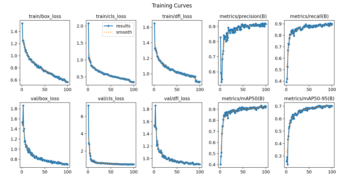
plots=True: Automatically generates result charts after training: loss curves, mAP curves, confusion matrix, and sample predictions. These are saved to the output folder and are the primary way to evaluate whether training worked correctly.

Output Settings

project='archery_yolo26' / name='v1' / exist_ok=True: Results save to archery_yolo26/v1/. Using name='v1' on the next run sends results to archery_yolo26/v1/ without overwriting. exist_ok=True means if v1 already exists it overwrites rather than erroring.

Hardware Settings

device=0: Use GPU 0 (the first GPU available). Without this it falls back to CPU.

workers=2: Number of CPU threads loading images in parallel while the GPU trains.

cache=True: Loads all training images into RAM at the start. After that, each epoch reads from RAM instead of disk, making training significantly faster. At ~500 images this fits comfortably in RAM.

---

Performance Metrics — What They Mean in This Context

Before looking at the numbers, it’s worth being precise about what each metric captures in this specific task.

Precision (Quality): When the model says “I found an arrow tip,” how often is it actually an arrow tip? A bounding box drawn around a hole in the target or a ring line and classified as arrow_tip lowers Precision.

Recall (Quantity): Of all the arrow tips actually on the target, how many did the model find? If there are 6 arrows on the target and the model only detects 4, Recall is 0.66 (66%).

mAP50 (Overall accuracy): Mean Average Precision at 0.5 IoU. A detection counts as correct if the predicted bounding box overlaps at least 50% with the ground truth box. This is the primary benchmark metric.

mAP50-95 (Localization strictness): The same metric averaged across IoU thresholds from 50% to 95%. This is much stricter and more meaningful for precise localization tasks, an arrow tip bounding box that’s roughly in the right region passes mAP50 but fails mAP50-95 if it’s not pixel-tight. For scoring arrows near ring boundaries, this number matters more than mAP50.

---

Performance Results & Full Analysis

Model Summary and Initial Validation

YOLO26s:

YOLO26s summary (fused): 122 layers, 9,466,728 parameters, 0 gradients, 20.5 GFLOPs

Class           Images  Instances   Box(P      R      mAP50   mAP50-95)
all                 50        624   0.908   0.870   0.912      0.698
arrow_shaft         50        267   0.893   0.816   0.914      0.795
arrow_tip           50        257   0.829   0.751   0.772      0.278
target_center       50         50   0.979   0.913   0.974      0.740
target_face         50         50   0.930   1.000   0.988      0.979

Speed: 0.3ms preprocess, 5.3ms inference, 0.0ms loss, 1.0ms postprocess per image

YOLOv12s:

YOLOv12s summary (fused): 159 layers, 9,232,428 parameters, 0 gradients, 21.2 GFLOPs

Class           Images  Instances   Box(P      R      mAP50   mAP50-95)
all                 50        624   0.911   0.890   0.924      0.705
arrow_shaft         50        267   0.934   0.899   0.949      0.818
arrow_tip           50        257   0.859   0.760   0.783      0.277
target_center       50         50   0.947   0.900   0.972      0.732
target_face         50         50   0.905   1.000   0.993      0.993

Speed: 0.2ms preprocess, 8.7ms inference, 0.0ms loss, 4.7ms postprocess per image

Validation Set Performance

Metric	YOLO26s	YOLOv12s
Overall mAP50	0.913	0.924
Overall mAP50-95	0.698	0.704
Precision	0.910	0.911
Recall	0.871	0.890

Per-Class mAP50:

Class	mAP50 (YOLO26s)	mAP50-95 (YOLO26s)	mAP50 (YOLOv12s)	mAP50-95 (YOLOv12s)
arrow_shaft	0.914	0.795	0.948	0.818
arrow_tip	0.776	0.278	0.785	0.277
target_center	0.975	0.742	0.972	0.732
target_face	0.989	0.980	0.993	0.993

Test Set Performance

Metric	YOLO26s	YOLOv12s
Overall mAP50	0.875	0.872
Overall mAP50-95	0.653	0.659
Precision	0.878	0.879
Recall	0.844	0.862

Per-Class mAP50:

Class	mAP50 (YOLO26s)	mAP50-95 (YOLO26s)	mAP50 (YOLOv12s)	mAP50-95 (YOLOv12s)
arrow_shaft	0.909	0.748	0.901	0.704
arrow_tip	0.673	0.195	0.608	0.186
target_center	0.951	0.717	0.985	0.769
target_face	0.969	0.954	0.992	0.977

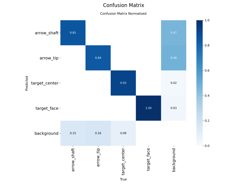
Confusion Matrices

YOLO26s

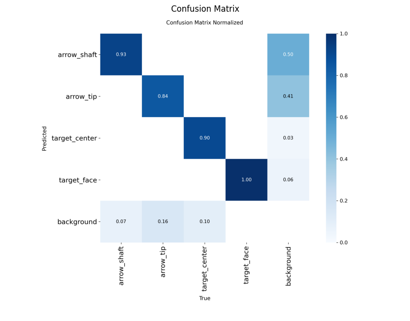
YOLOv12s

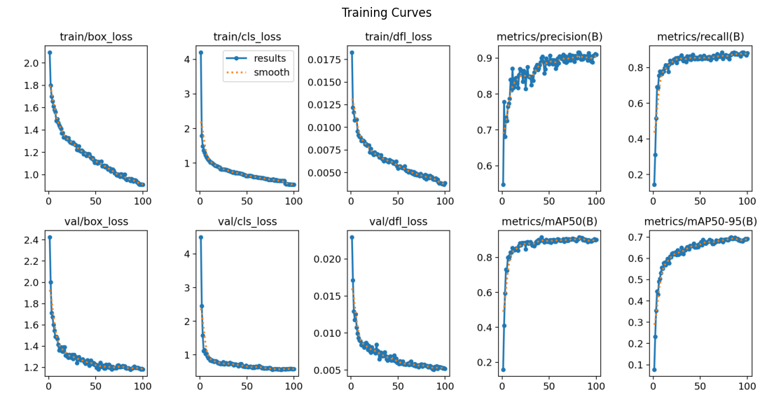
Training Curves

YOLO26s

YOLOv12s

Comparative Analysis

Validation vs. Test Gap:

YOLO26s:
  Val  mAP50: 0.913
  Test mAP50: 0.875
  Gap:        0.038

YOLOv12s:
  Val  mAP50: 0.924
  Test mAP50: 0.872
  Gap:        0.053

YOLOv12s scores higher on validation but has a larger validation-to-test gap (0.053 vs 0.038), indicating more overfitting. On the held-out test set, the two models are essentially tied on overall mAP50.

Critical Class: Arrow Tip Detection

Metric	YOLO26s	YOLOv12s
Arrow Tip mAP50 (test)	0.673	0.608
Arrow Tip mAP50-95 (test)	0.195	0.186
Localization gap	0.478	0.422

This is the deciding metric. Arrow tips are the only class that directly determines scores. YOLO26s outperforms YOLOv12s on the test set for the most critical class. Missing a tip means a missed score, there is no worse failure mode for this application.

Inference Speed:

Model	Total inference
YOLO26s	6.3ms
YOLOv12s	13.4ms

YOLO26s is approximately 2× faster end-to-end.

Model Selection: YOLO26s was selected for production based on superior arrow tip detection performance and significantly lower latency. YOLOv12s’s better target_center localization (0.985 vs 0.951 mAP50) was noted but outweighed by the tip detection advantage.

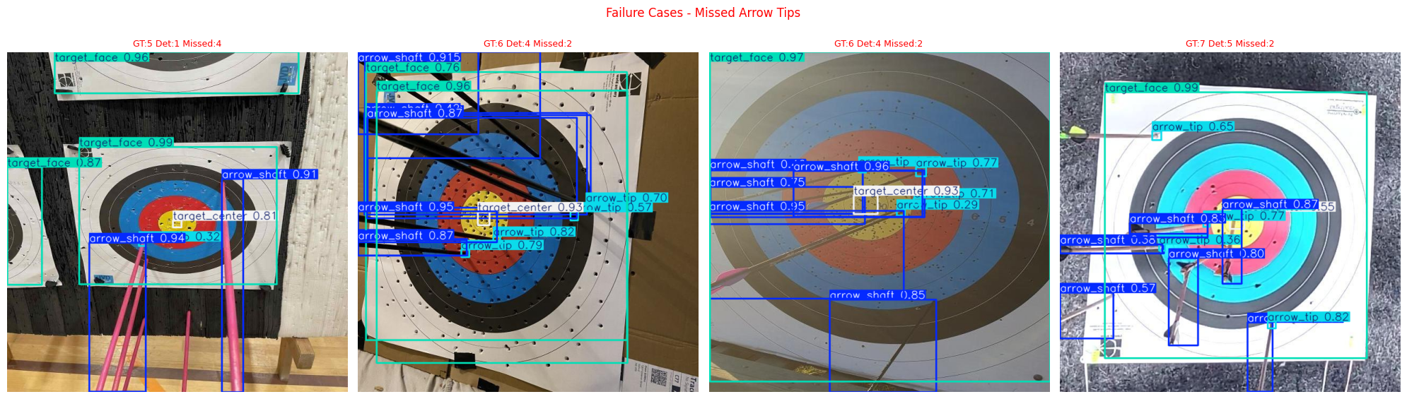
Failure Case Analysis

YOLO26s — 9/25 test images with missed arrow tips:

Image	GT Arrows	Detected	Missed
135_jpeg_jpg.rf.25c9c1679a…	5	1	4
IMG_3836_result_jpg.rf.e8c2…	6	4	2
20250619_162850_jpg.rf.014b…	6	4	2
112_countarrow_poly_png_jpg…	7	5	2
14_countarrow_poly_png_jpg…	2	1	1

YOLOv12s — 7/25 test images with missed arrow tips:

Image	GT Arrows	Detected	Missed
135_jpeg_jpg.rf.25c9c1679a…	5	2	3
IMG_3764_result_jpg.rf.cc8a…	6	4	2
20250619_162850_jpg.rf.014b…	6	4	2
20250927_101828_jpg.rf.a615…	6	5	1
20250913_104221_jpg.rf.851a…	6	5	1

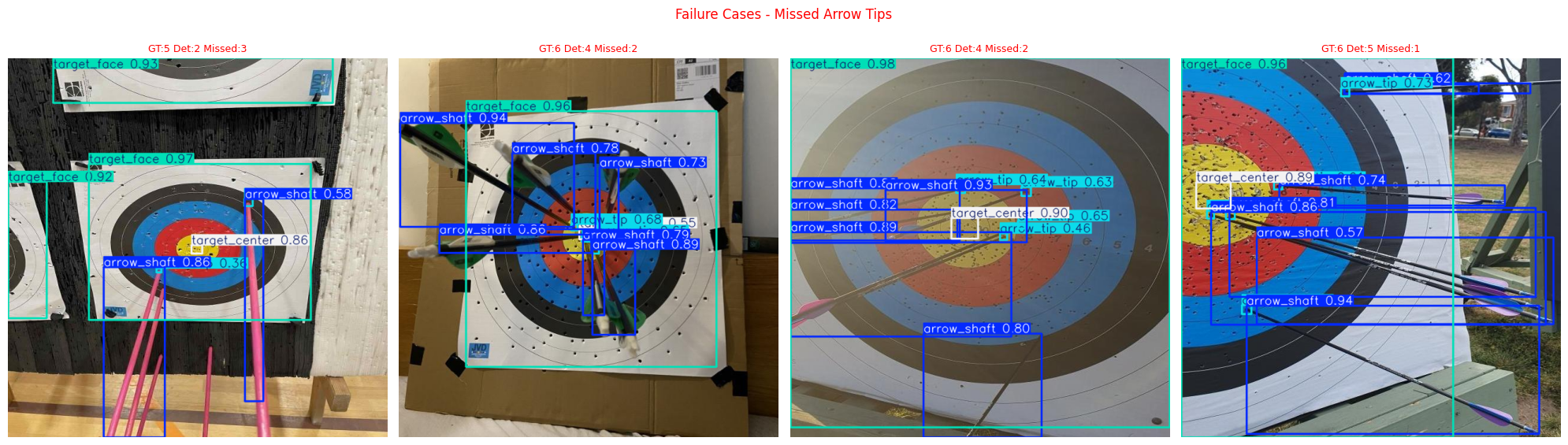
The primary failure mode is identical for both models: dense clustering with 5+ arrows. Every worst-case failure involves multiple arrows packed together. Images with fewer than 4 arrows showed near-perfect detection across both models.

Key Insights

1. Generalization is strong. The 3.8% validation-to-test gap for YOLO26s indicates the model is learning genuine features rather than memorizing training examples.

2. Target detection is reliable. Both target_face and target_center exceed 95% mAP50 on the unseen test set. The scoring geometry anchor points are found consistently regardless of shooting distance, lighting, or camera angle.

3. Arrow tip localization is the primary limitation. The localization gap is sharp: 67.3% mAP50 but only 19.5% mAP50-95 — a 47.8 point drop. The model finds approximate tip regions but struggles with pixel-precise localization. For arrows near ring boundaries, this directly translates to incorrect scores.

4. Clustering degrades performance. The primary failure mode is clear and actionable: 5+ arrows clustered. This is a data problem as much as a model problem, the training set needs more examples of dense cluster scenarios.

5. Inference is fast enough. At 6.3ms per image on GPU, the model is well within real-time requirements for a mobile app where images are processed once per end.

---

Scoring Logic & Integration Pipeline

Detection is only half the problem. Once YOLO26s returns bounding box coordinates, they are processed by a custom geometric engine that converts pixel positions into scores.

Image → Perspective Correction → YOLO Detection → Geometry Resolution → Score Calculation → Visualization

Project Structure

archery/
├── models/
│   └── best.pt
├── src/
│   ├── visualize_inference.py   # drawing results for single inference
│   ├── detection.py             # YOLO inference
│   ├── perspective.py           # HSV + ellipse + affine warp
│   ├── geometry.py              # distance calc + score lookup
│   └── visualize.py             # drawing results
├── main.py                      # entry point
├── labeling.py                  # auto-label new images using model
└── config.py                    # all constants and paths

The pipeline operates entirely in pixel coordinates. Every module produces and consumes pixel-space values. This eliminates the normalization mismatch that is common in systems that mix YOLO’s 0–1 normalized outputs with pixel-space geometry.

---

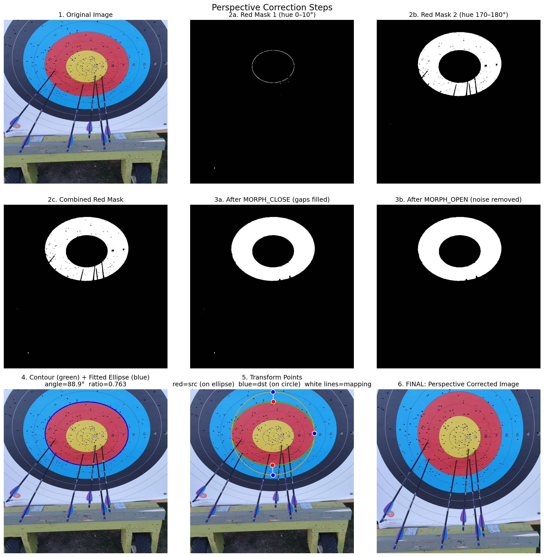
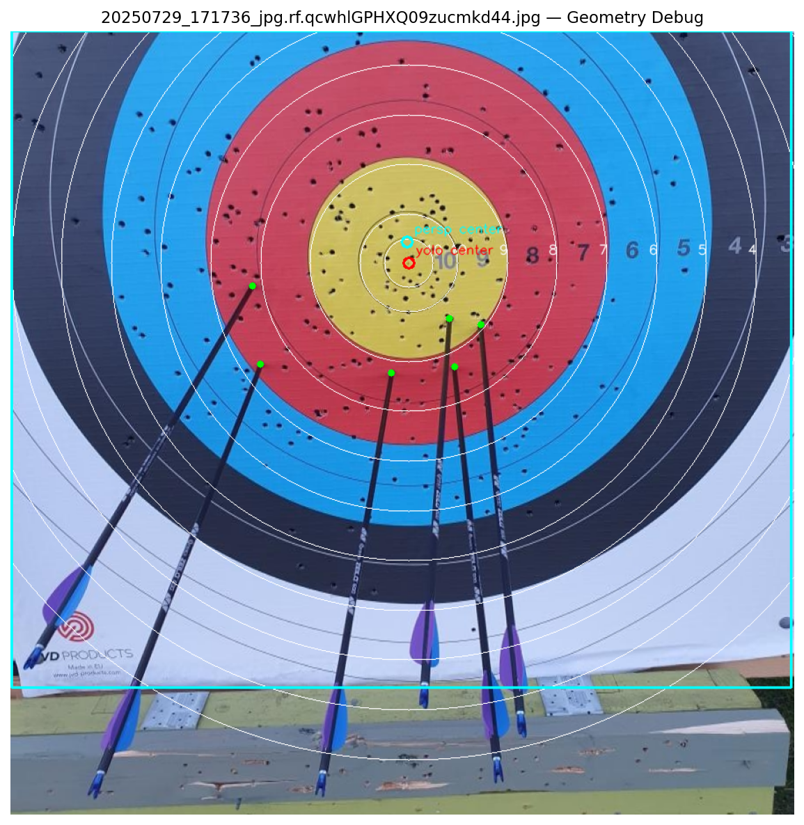
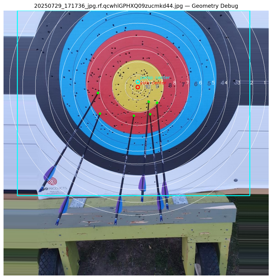
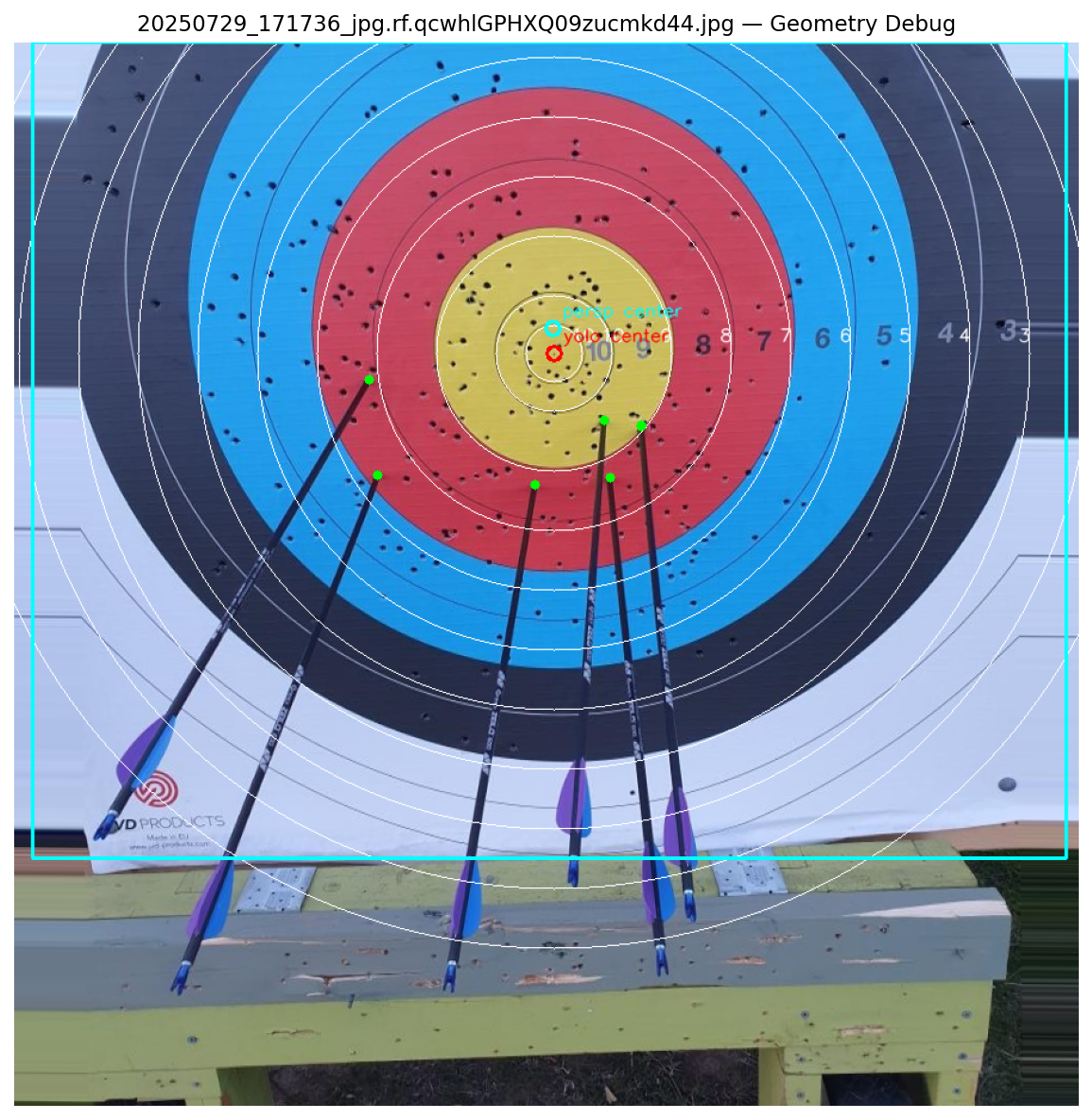
Stage 1 — Perspective Correction (perspective.py)

Photographs of archery targets are rarely taken head-on. Camera tilt causes the circular target to appear as an ellipse in the image. If scoring directly on the tilted image, arrows near the edges receive systematically wrong scores because distances are compressed along the tilt axis. Perspective correction warps the image so the target becomes circular again, restoring true radial distances.

Step 1.1 — Red Zone Isolation via HSV Color Space

The red scoring zone (rings 7 and 8) provides a reliable structural marker because red is the most chromatically distinct color on a WA target face. The image is converted from BGR to HSV (Hue, Saturation, Value) because red pixels cluster tightly in hue space, making them easier to isolate than in RGB where red is spread across all three channels.

Red wraps around the hue cylinder in HSV (0° and 360° are both red), so we use two separate hue ranges to capture it completely:

# Range 1: hue 0–10° (orange-red end)
RED_HSV_LOWER_1 = (0,   80, 80)
RED_HSV_UPPER_1 = (10,  255, 255)

# Range 2: hue 170–180° (magenta-red end)
RED_HSV_LOWER_2 = (170, 80, 80)
RED_HSV_UPPER_2 = (180, 255, 255)

The saturation and value thresholds ($S \geq 80$, $V \geq 80$) reject whitish and dark pixels that might have a red-ish hue due to noise. The two binary masks are combined with cv2.bitwise_or to produce a single red mask as shown in Figure 8 plot 2.

Step 1.2 — Morphological Cleanup

The raw red mask contains noise (small red-ish artifacts outside the target) and gaps (where arrows, text, or shadows occlude the red ring). Then apply two morphological operations using a 7×7 kernel:

1. MORPH_CLOSE (dilation → erosion): Fills small holes inside the red region. Arrow shafts crossing the red zone create thin black lines in the mask; closing seals them as shown in Figure 8 plot 3a.
2. MORPH_OPEN (erosion → dilation): Removes small noise outside the red region. Stray red pixels from fletchings, clothing, or background objects are eliminated as shown in Figure 8 plot 3b.

The order matters: closing first preserves the red zone’s shape before opening trims exterior noise.

Step 1.3 — Contour Extraction and Ellipse Fitting

The external contours are then extracted from the cleaned mask using cv2.findContours and select the largest contour by area, this is the red scoring zone. OpenCV’s cv2.fitEllipse fits a rotated ellipse to this contour using least-squares optimization, returning three parameters:

• center $(c_x, c_y)$: the ellipse center in pixel coordinates
• axes $(w, h)$: the full width and height of the ellipse
• angle $\theta$: rotation angle in degrees

The aspect ratio (semi-minor / semi-major) tells us how much perspective distortion exists. A ratio of 1.0 means the target is already perfectly circular; lower values indicate more tilt.

Step 1.4 — Affine Warp (Ellipse → Circle)

To correct the perspective, I compute an affine transformation that maps the detected ellipse onto a circle. The output circle has a radius equal to the ellipse’s semi-major axis (the larger half-axis), preserving the maximum resolution.

The transformation requires three point correspondences. I choose the points that represent the true vertical and horizontal extrema of the rotated ellipse: the topmost, rightmost, and bottommost points.

The ellipse boundary in image coordinates uses a parametric form with rotation angle $\phi$:

$x(t) = c_x + a\cos t \cos\phi - b\sin t \sin\phi$ $y(t) = c_y + a\cos t \sin\phi + b\sin t \cos\phi$

where $a$ and $b$ are the semi-major and semi-minor axes, respectively.

To find the top/bottom points, I set the vertical derivative to zero:

$\frac{dy}{dt} = -a\sin t\,\sin\phi + b\cos t\,\cos\phi = 0$ $\quad \Rightarrow \quad \tan t_y = \frac{b\cos\phi}{a\sin\phi}$

To find the left/right points, I set the horizontal derivative to zero:

$\frac{dx}{dt} = -a\sin t\,\cos\phi - b\cos t\,\sin\phi = 0$ $\quad \Rightarrow \quad \tan t_x = -\frac{b\sin\phi}{a\cos\phi}$

In code these are computed robustly with arctan2:

t_y = np.arctan2(b * np.cos(phi), a * np.sin(phi))
t_x = np.arctan2(-b * np.sin(phi), a * np.cos(phi))

Each angle produces two extrema on the ellipse separated by $\pi$ radians, so I evaluate both $t$ and $t + \pi$ and choose:

• top as the point with minimum $y$
• right as the point with maximum $x$
• bottom as the point with maximum $y$

These are then paired with the corresponding circle points:

Point	Source (on ellipse)	Destination (on circle)
Top	Rotated ellipse top extremum	$(c_x, c_y - r)$
Right	Rotated ellipse right extremum	$(c_x + r, c_y)$
Bottom	Rotated ellipse bottom extremum	$(c_x, c_y + r)$

The 2×3 affine matrix $M$ is computed via cv2.getAffineTransform(src, dst) and applied to the entire image using cv2.warpAffine. After warping, the target face appears circular and all radial distances are geometrically correct.

Step 1.5 — Full Target Radius Estimation

The detected ellipse corresponds only to the red zone, not the full target. On a standard WA 122cm outdoor target, the red zone (rings 7–8) extends to 40% of the total target radius. A configurable ratio (RED_ZONE_RATIO = 0.4) is used to scale up:

$R_{\text{full}} = \frac{r_{\text{red zone}}}{\text{RED\_ZONE\_RATIO}}$

The center coordinates are also updated to account for the affine transformation by transforming the original center point through the same matrix $M$.

The function returns:

• The warped image (target is now circular)
• The affine matrix $M$
• A target dict {cx, cy, radius} in pixels, the estimated center and full target radius in the corrected image

Observations and Other Approaches

This stage was one of the most challenging parts of the project because it directly affects the accuracy of all later stages. Several approaches were tested beyond the affine warp described above.

Issues encountered:

• After warping, the ellipse center could be significantly offset from the YOLO-detected target_center, which proved more reliable. For that reason, the pipeline prioritizes the YOLO target center over the ellipse center.
• Some images produced perfect results while others missed arrows entirely. Further debugging showed that the full target radius estimated from the red-zone ellipse was not accurate enough. A small radius error propagated outward through each ring, causing the warped outer rings to deviate significantly from their true positions.

Approaches tested to fix the radius issue:

• Major axis as radius: The initial approach, produces the described propagation error.
• Minor axis as radius: The output still suffered from the same distortion; only the warped scale changed.

• Average of both axes: Same class of error, the propagation remained.

• Full homography (4 points): Replaced the affine transform with cv2.getPerspectiveTransform(src_pts, dst_pts), adding the leftmost circle point as a fourth correspondence. The same propagated error remained.

• Point selection variation: I suspected the three or four point correspondences might be too geometrically similar when aligned with the major axis. However, changing the radius assumption to the axis average didn’t improve the result, so that hypothesis appeared unlikely.

This remains an open problem. The pipeline currently compensates by using YOLO’s target_center as the primary center reference and the target_face bounding box as a radius fallback, but robust perspective correction is still needed for the outer rings.

---

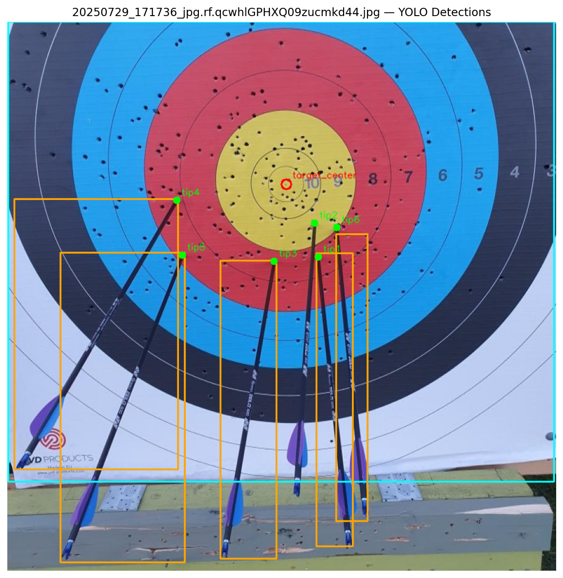
Stage 2 — YOLO Detection(detection.py)

The YOLO26s model runs on the perspective-corrected image and detects four object classes:

Class	Purpose	Output Used
arrow_tip	Point of impact	Center $(c_x, c_y)$ for scoring
arrow_shaft	Arrow body	Used to refine tip position via shaft direction
target_center	The X-ring / 10-ring bullseye	Provides precise center reference
target_face	Full target boundary	Fallback for radius estimation

All coordinates are returned in pixel space using box.xywh (not normalized box.xywhn), so they can be directly compared with the pixel-space geometry from Stage 1.

The model runs with conf=0.25, iou=0.45, and max_det=20. For target_face and target_center, only the highest-confidence detection is kept. All arrow_tip and arrow_shaft detections are collected into lists.

---

Stage 3 — Geometry Resolution (geometry.py)

The geometry resolver determines the best center and best radius for scoring by fusing information from the two independent sources: perspective correction (HSV-based) and YOLO detection.

Center Selection Priority:

1. YOLO target_center (highest priority): The model detects a tight bounding box around the X-ring; its center point is the most spatially precise locator available.
2. Ellipse center (from perspective.py): The centroid of the fitted red zone ellipse, transformed through the affine warp matrix.
3. YOLO target_face center (fallback): The center of the full target bounding box; least precise but still functional.

Radius Selection Priority:

1. Ellipse-based radius (highest priority): Already scaled by RED_ZONE_RATIO to represent the full target radius.
2. YOLO target_face width / 2 (fallback): Uses the face bounding box as an approximation of the target diameter.

Cross-Validation: When both sources provide a center, the resolver computes the Euclidean distance between them. If the mismatch exceeds 30 pixels, a warning is logged, this can indicate that the perspective correction drifted or that the YOLO detection is inaccurate.

---

Stage 4 — Score Calculation (geometry.py)

Arrow Tip Refinement

YOLO’s bounding boxes have limited localization precision for small objects like arrow tips (mAP50-95 of only 19.5%). To compensate, each tip’s position is refined using its associated arrow shaft:

1. For each detected tip, find the nearest shaft by Euclidean distance.
2. If the nearest shaft is within 50 pixels, use it, otherwise it likely belongs to a different arrow.
3. Compute a refined position by projecting along the shaft’s direction (estimated from its bounding box aspect ratio) to the shaft’s far endpoint.
4. Weighted blend the original tip position with the shaft-refined position:

$P_{\text{final}} = P_{\text{tip}} \cdot w + P_{\text{shaft}} \cdot (1 - w)$

where $w$ is the tip’s detection confidence. High-confidence tips are trusted more; low-confidence tips defer to shaft geometry.

Distance Ratio Computation

For each refined tip position $(t_x, t_y)$:

$d = \sqrt{(t_x - c_x)^2 + (t_y - c_y)^2}$

$\text{ratio} = \frac{d}{R_{\text{full}}}$

This ratio is target-size-invariant: 0.0 is dead center (X-ring), 1.0 is the outer edge of ring 1, and values above 1.0 are misses. The angle $\alpha = \text{atan2}(t_y - c_y, t_x - c_x)$ captures the clock direction, which is useful for placing arrows on a clean target diagram in the app.

Ring Lookup

The ratio is compared against the WA 122cm ring table:

Ring	Outer Edge Ratio	Score
X	0.05	10
10	0.10	10
9	0.20	9
8	0.30	8
7	0.40	7
6	0.50	6
5	0.60	5
4	0.70	4
3	0.80	3
2	0.90	2
1	1.00	1
Miss	> 1.0	0

The first ring whose outer edge ratio exceeds the tip’s ratio determines the score. Note that both the inner X-ring and the outer 10-ring score 10 points, matching WA rules.

Boundary Detection

Arrows landing near ring boundaries are the most common source of scoring disputes. The system flags any arrow whose ratio falls within ±0.015 (the BOUNDARY_TOLERANCE) of any ring edge. These arrows are marked is_boundary: true in the output and displayed with a cyan warning border in the visualization. This alerts the user that manual verification may be needed.

---

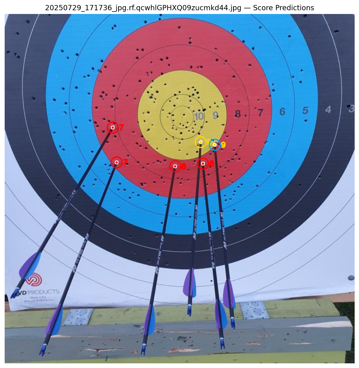
Stage 5 — Visualization (visualize.py)

The final stage renders scoring results on the perspective-corrected image:

• Concentric ring overlays: The full target radius, red zone boundary, black zone boundary, and white zone boundary are drawn as circles centered on the resolved center point. These should visually align with the actual rings on the target.
• Arrow shaft boxes: Orange rectangles around detected shafts.
• Scored arrow markers: Each tip is drawn as a filled circle colored by its score, gold for 10/9, red for 8/7, blue for 6/5, black for 4/3, white for 2/1, gray for miss. The numeric score is displayed next to each marker.
• Boundary warnings: Tips near ring edges get an cyan border ring, providing visual indication of scoring uncertainty.

---

Stage 6 — Output

The pipeline returns a structured dictionary:

{
    'image': 'filename.jpg',
    'arrows': [
        {'score': 10, 'ratio': 0.0312, 'angle': 45.2, 'is_boundary': False,
         'x': 412.3, 'y': 438.1, 'confidence': 0.87},
        ...
    ],
    'total': 58,
    'arrow_count': 6,
    'boundaries': [3]   # indices of arrows near ring edges
}

---

Limitations, Known Issues & What’s Next

Current Limitations

Arrow tip detection degrades when 5+ arrows cluster in high-scoring zones. This is the single most impactful failure mode and is fundamentally a data problem, the training set has too few examples of dense cluster scenarios.

Localization precision is insufficient for tournament-grade scoring without user confirmation. An mAP50-95 of 19.5% on arrow tips means the model’s bounding boxes are often not tight enough to make confident calls near ring boundaries. The boundary flagging system compensates, but manual verification is still required for those cases.

The model was trained on ~500 images. Performance is expected to improve substantially with more diverse training data, particularly close-up images of clustered arrows in the gold zone.

Perspective correction is fragile for some camera angles. Small errors in the red-zone ellipse radius estimate propagate outward through the ring table. The pipeline compensates by preferring YOLO-detected centers over ellipse-derived ones, but the full correction pipeline remains brittle on difficult angles.

What’s Next

• Collect 200–300 more images specifically targeting densely clustered arrows
• Explore keypoint detection models (predicting the tip as a point rather than a bounding box center) to improve mAP50-95
• Investigate more robust perspective correction approaches, potentially using target_face YOLO detection as the primary geometric anchor rather than the HSV ellipse
• Add support for indoor 40cm and triple-spot target faces
• Investigate detecting full ring contours (not only the red zone), fit them jointly, and use the averaged fit for a more robust center and radius estimate.

---

References

1. Roboflow Dataset 1 — Archery-skmsa

2. Roboflow Dataset 2 — Uni-oidi4

3. Roboflow Dataset 3 — Archery-scoring

4. Roboflow Dataset 4 — Shrutiharshil

5. Roboflow Dataset 5 — Final Dataset

6. YOLO26 Docs — Ultralytics YOLO26

7. YOLO12 Docs — Ultralytics YOLO12